The kernel estimator is a sum of “bumps” placed at the observations.
- The kernel function $K$ determines the shape of the bumps.
- The window width $h$ determines their width.
Consider random variable $X$ that has PDF $f$ $$ P(a < X < b) = \int_{a}^{b} f(x) dx, \quad \text{for all } a < b. $$
Known: A set of observed data points sample from an unknow PDF.
This book focuses on nonparametric approach.
Given
The bins of the histogram is the intervals $[x_0 + mh, x_0 + (m + 1)h]$ for $m \in \mathbb{Z}$.
The histogram
a priori bining: the bin boundaries are determined before observing the data.
Data-Dependent Binning: This method involves determining the bin boundaries based on the observations
If the random variable $X$ has density $f$, then $$ f(x) = \lim_{h \to 0} \frac{1}{2h} P(x - h < X < x + h). $$
We have an x and we’re looking for its neighbours in a $2h$ bin.
For any given $h$, we can estimate $P(x - h < X < x + h)$ by the proportion of the sample falling in the interval $(x - h, x + h)$. Thus a natural estimator $\hat{f}$ of the density is given by choosing a small number $h$
Define the weight function $$ w(x) = \begin{cases} \frac{1}{2}, & \text{if } |x| < 1 \\ 0, & \text{otherwise} \end{cases} $$
This weight function serves as a simple indicator function that determines whether a given point $x$ should contribute to the density estimate.
Then
Replace the weight function $w$ by a kernel function $K$ such that $$ \int_{-\infty}^{\infty} K(x) \, dx = 1. $$
Usually but not always, $K$ will be a symmetric PDF (normal, for instance).
The kernel estimator with kernel $K$
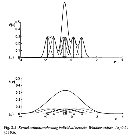
The kernel estimator is a sum of “bumps” placed at the observations.
In KDE, the bandwidth (or window width) is fixed across the entire data sample. This causes issues when the data has a long tail, as smaller densities in the tails may create spurious noise in the estimated density function.