Complexity of the clique tree is exponential in the tree-width of the network $ \rightarrow $ exact algorithms become infeasible for networks with a large tree-width.
Exact Inference Revisited
Casting exact inference as an optimization problem.
Given factorized distribution
$$
P_{\Phi} (\mathcal{X}) = \frac{1}{Z} \prod_{\phi \in \Phi} \phi(U_\phi)
$$
- $ U_\phi = Scope[\phi] \subseteq \mathcal{X} $: the scope of each factor.
Goal: Answering queries about $ P_{\Phi} $
- Marginal probabilities of variables,
- partition function $ Z $.
Recall:
- Clique tree BP results in a calibrated cluster tree $ \Rightarrow $ all pairs of adjacent cliques are calibrated (by definition).
- Calibrated set of beliefs $ Q $ for the cluster tree represents a distribution $ P_\Phi (\mathcal{X}) $.
ℹ️
Can view Exact Inference as searching for a calibrated
distribution $ Q $ that matches $ P_\Phi \rightarrow $ minimizes relative entropy $ \mathbb{D}(Q || P_\Phi) $
CTree-Optimize-KL
Given a set of beliefs
$$
Q = \{ \beta_i : i \in V_{\mathcal{T}} \} \cup \{ \mu_{i,j} : (i-j) \in E_{\mathcal{T}} \}
$$
- $ \mathcal{T} $: clique tree structure for $ P_\Phi $.
- $ \beta_i $: beliefs over cluster $ C_i $.
- $ \mu_{i, j} $: beliefs over sepset $ S_{i, j} $.
The set of beliefs in $ T $ defines a distribution $ Q $ due to the calibration requirement:
$$
\boxed{ Q(\mathcal{X}) = \frac{\prod_{i \in V_{\mathcal{T}}} \beta_i}{\prod_{(i - j) \in E_{\mathcal{T}}} \mu_{i, j}} }
$$
Calibration requirement ensures $ Q $ statisfies the marginal consistency constrants: For each $ (i - j) \in E_{\mathcal{T}} $, the beliefs on $ S_{i, j} $ are the marginal of $ B_i $ (and $ B_j $).
$$
\mu_{i, j} (S_{i, j}) = \sum_{C_i - S_{i, j}} \beta_i (C_i) = \sum_{C_j - S_{i, j}} \beta_j (C_j)
$$
From Theorem 10.4
$$
\beta_i[c_i] = Q(c_i)
$$
$$
\mu_{i, j}[s_{i, j}] = Q(s_{i, j})
$$
CTree-Optimize-KL
Find $ Q = \{ \beta_i : i \in V_{\mathcal{T}} \} \cup \{ \mu_{i,j} : (i-j) \in E_{\mathcal{T}} \} $
Maximizing $ - \mathbb{D} (Q || P_\Phi) $
subject to
$$
\mu_{i, j} (s_{i, j}) = \sum_{C_i - S_{i, j}} \beta_i (c_i) \quad \forall (i - j) \in E_T, \forall s_{i, j} \in Val(S_{i, j})
$$
$$
\sum_{c_i} \beta_i (c_i) = 1 \quad \forall i \in V_T
$$
- if $ \mathcal{T} $ is a proper cluster tree for $ \Phi $, there is a set $ Q $ that induces a distribution $ Q = P_\Phi $.
- Because this solution achieves a relative entropy of 0, which is the highest value possible, it is the unique global optimum of this optimization.
Theorem 11.1
If $ \mathcal{T} $ is an I-map of $ P_\Phi $, then there is a unique solution to CTree-Optimize-KL.
Exact Inference as Optimization
- In Chapter 10, Belief Propagation results in a calibrated clique tree $ \rightarrow Q = P $.
- In this chapter, we are no longer in a clique tree but rather in a general cluster graph, which can have loops.
- Can’t use the clique tree message passing algorithm $ \rightarrow $ can’t guarantee calibrated tree: $ Q \not= P $
Goal:
- Introduce a set of approximate beliefs $ Q = \{ \beta_i(C_i), \mu_{ij} (S_{ij}) \} $.
- try to make $ Q $ as close as possible to $ P $.
- by optimizing the energy function.
The Energy Functional
functional?
Functions
- Input: variables
- Output: a value
- Full and partial derivatives $ \frac{df}{dx} $
- E.g. Maximize likelihood $ p(x \mid \theta) $ w.r.t. parameters $ \theta $
Functional
- Input: functions
- Output: a value
- Functional derivatives $ \frac{\delta F}{\delta f} $
- E.g., Maximize the entropy $ H[p(x)] $ w.r.t. p(x)
Theorem 11.2
$$
\boxed{ \mathbb{D} (Q || P_\Phi) = \ln Z - F[\tilde{P}_\Phi, Q] }
$$
where $ F[\tilde{P}_\Phi, Q] $ is the energy functional
$$
\begin{align*}
F[\tilde{P}_\Phi, Q] &= E_Q[\ln \tilde{P}(\mathcal{X})] + H_Q(\mathcal{X})
\end{align*}
$$
$$
= \sum_{\phi \in \Phi} E_Q [\ln \phi] + H_Q(\mathcal{X})
$$
- $ \sum_{\phi \in \Phi} E_Q [\ln \phi] $: energy term
- Each $ \phi $ appears as a seperate term.
- If factors $ \phi $ that comprise $ \Phi $ are small, each expectation deals with relatively few variables.
- Depends on $ Q $.
- Inference is “easy” in $ Q \rightarrow $ evaluate such expectations easy.
- $ H_Q(\mathcal{X}) $: entropy term
- Depends on $ Q $.
- involving the entropy of an entire joint distribution; thus, it cannot be tractably optimized.
Proof
$$
\mathbb{D} (Q || P_\Phi) = E_Q[\ln Q (\mathcal{X})] - E_Q[\ln P_\Phi (\mathcal{X})]
$$
- $ H_Q (\mathcal{X}) = - E_Q[\ln Q (\mathcal{X})] $.
- $ P_\Phi (\mathcal{X}) = \frac{1}{Z} \sum_{\phi \in \Phi} \phi \Rightarrow \ln P_\Phi = \sum_{\phi \in \Phi} \ln \phi - \ln Z $.
Thus,
$$
\mathbb{D} (Q || P_\Phi) = - H_Q (\mathcal{X}) - E_Q \left[ \sum_{\phi \in \Phi} \ln \phi \right] + E_Q[\ln Z]
$$
$$
= -F[\tilde{P}_\Phi, Q] + \ln Z
$$
ℹ️
Minimizing the relative entropy $ \mathbb{D} (Q || P_\Phi) $ is equivalent to maximizing the energy functional $ F[\tilde{P}_\Phi, Q] $.
Optimizing the Energy Functional
Since $ \mathbb{D} (Q || P_\Phi) $,
$$
\ln Z \geq F[\tilde{P}_\Phi, Q]
$$
- $ F $ is a lower bound on $ \ln Z $.
- Recall: in directed models, $ Z = P(E) \rightarrow $ the hardest part of inference,
- if $ \mathbb{D} (Q || P_\Phi) $ is small $ \rightarrow $ get a good lower-bound approximation to $ Z $.
Variational Methods
Inference methods that can be viewed as strategies for optimizing the energy functional.
Variatioinal Analysis
The exact energy functional
$$
F[\tilde{P}_\Phi, Q]
$$
has terms involving the entropy of an entire joint distribution; thus, it cannot be tractably optimized $ \rightarrow $ factored energy functional
$$
\tilde{F}[\tilde{P}_\Phi, Q]
$$
defined in terms of entropies of clusters and sepsets, which can be computed efficiently based purely on local information at the clusters.
Marginal polytope
- $ U $: cluster graph
- $ P $: distribution
The marginal polytope is the set of all cluster (and sepset) beliefs that can be obtained from marginalizing an actual distribution $ P $
- set of marginals obtained from the polytope of all probability distributions over $ \mathcal{X} $.
$$
Marg[U] = \{ Q_P: P \text{ is a distribution over } \mathcal{X} \}
$$
that is
$$
Q_P = \{ P(C_i): i \in V_U \} \cup \{ P(S_{i, j}): (i-j) \in E_U \}
$$
Factored energy functional
𐰋𐰍𐰃𐰤
$$
\tilde{F}[\tilde{P}_{\Phi}, Q]
$$
$$
= \boxed{ \sum_{i \in V_{\mathcal{T}}} E_{C_i \sim \beta_i}[\ln \psi_i] +
\sum_{i \in V_{\mathcal{T}}} H_{\beta_i}(C_i) -
\sum_{(i-j) \in E_{\mathcal{T}}} H_{\mu_{i,j}}(S_{i,j}) }
$$
- $ \alpha $: maps $ \phi \in \Phi \mapsto $ cluster $ C_i \in \mathcal{T} $.
- $ E_{C_i \sim \beta_i}[\ln \psi_i] $: Expectation on the value $ C_i $ given the beliefs $ \beta_i $.
- $ \psi_i: Val(C_i) \mapsto \mathbb{R} $: initial potential of $ C_i $
$$
\psi_i = \prod_{\phi, \alpha (\phi) = i} \phi
$$
⚠️
In this reformulation, all the terms are local (refer to a specific belief factor).
Proof
- $ \ln \psi_i = \sum_{\phi, \alpha (\phi) = i} \ln \phi $.
- $ \beta_i(c_i) = Q(c_i) $.
Thus,
$$
\sum_{\phi \in \Phi} E_Q [\ln \phi] = \sum_{i \in V_{\mathcal{T}}} E_{C_i \sim \beta_i}[\ln \psi_i]
$$
Recall
$$
H_Q (\mathcal{X}) = E_Q \left[ \ln \frac{1} {Q(\mathcal{X})} \right]
$$
$$
Q(\mathcal{X}) = \frac{\prod_{i \in V_{\mathcal{T}}} \beta_i}{\prod_{(i - j) \in E_{\mathcal{T}}} \mu_{i, j}}
$$
Take the logarithm
$$
\ln Q(\mathcal{X}) = \sum_{i \in V_T} \ln \beta_i(c_i) - \sum_{(i-j) \in E_T} \ln \mu_{i,j}(s_{i,j})
$$
Compute entropy
$$
H_Q(\mathcal{X}) = - E_Q \left[ \sum_{i \in V_T} \ln \beta_i(c_i) - \sum_{(i-j) \in E_T} \ln \mu_{i,j}(s_{i,j}) \right]
$$
Thus,
$$
H_Q (\mathcal{X}) = \sum_{i \in V_{\mathcal{T}}} H_{\beta_i}(C_i) -
\sum_{(i-j) \in E_{\mathcal{T}}} H_{\mu_{i,j}}(S_{i,j})
$$
CTree-Optimize
In calibrated clique tree, we get marginal consistency for free, however in a loopy graph, running message passing does not necessarily give calibrated beliefs.
- Trick: even though consistency doesn’t happen naturall $ \rightarrow $ force it by adding it as a constraint in the optimization problem.
Find $ Q = \{ \beta_i : i \in V_{\mathcal{T}} \} \cup \{ \mu_{i,j} : (i-j) \in E_{\mathcal{T}} \} $
Maximizing $ \tilde{F}[\tilde{P}_{\Phi}, Q] $
subject to
$$
\mu_{i, j} [s_{i, j}] = \sum_{C_i - S_{i, j}} \beta_i(c_i) \quad \forall (i - j) \in E_T, \forall s_{i, j} \in Val(S_{i, j}) \quad \text{(Marginal consistency)}
$$
$$
\sum_{c_i} \beta_i (c_i) = 1 \quad \forall i \in V_T \quad \text{(Normalization)}
$$
$$
\beta_i (c_i) \geq 0 \quad \forall i \in V_T, c_i \in Val(C_i) \quad \text{(Non-negativity)}
$$
Fixed point Characterization
- Stationary point: either a local maximum, a local minimum or a saddle point.
- CTree-Optimize has a single global maximum (theorem 11.1).
- Can show that it is also the only stationary point $ \rightarrow $ once we find a stationary point, we know that its the maximum.
Goal: Maximizing $ \tilde{F}[\tilde{P}_{\Phi}, Q] $ under consistency constraints.
Abt the Non-negativity constraint: Do not need to enforce this explicitly because the assumption that factors are strictly positive implies the beliefs will be nonnegative.
$ \Rightarrow $ Lagrange multiplier
$$
J = \tilde{F}[\tilde{P}_{\Phi}, Q]
$$
$$
-\sum_i \lambda_i \left( \sum_{c_i} \beta_i (c_i) - 1 \right)
$$
$$
-\sum_i \sum_{j \in Nb_i} \sum_{s_{i, j}} \lambda_{i \to j} [s_{i, j}] \left( \sum_{c_i \sim s_{i, j}} \beta_i (c_i) - \mu_{i, j} [s_{i, j}] \right).
$$
Taking derivatives of $ J $ w.r.t
- $ \beta_i (c_i) $
- $ \mu_{i, j}[s_{i, j}] $
$$
\frac{\partial J}{\partial \beta_i (c_i)} = \ln \psi_i [c_i] - \ln \beta_i (c_i) - 1 - \sum_{j \in Nb_i} \lambda_{i \to j} [s_{i, j}]
$$
$$
\frac{\partial J}{\partial \mu_{i, j} [s_{i, j}]} = \ln \mu_{i, j} [s_{i, j}] + 1 + \lambda_{i \to j} [s_{i, j}] + \lambda_{j \to i} [s_{i, j}]
$$
explain
$$
\tilde{F}[\tilde{P}_{\Phi}, Q]
$$
$$
= \sum_{i \in V_{\mathcal{T}}} E_{C_i \sim \beta_i}[\ln \psi_i] +
\sum_{i \in V_{\mathcal{T}}} H_{\beta_i}(C_i) -
\sum_{(i-j) \in E_{\mathcal{T}}} H_{\mu_{i,j}}(S_{i,j})
$$
Recall: $ X \sim P \rightarrow E_{X \sim P} [g(X)] = \sum_x P(x) \cdot g(x) $
- $ E_{C_i \sim \beta_i} [\ln \psi_i] = \sum_{c_i} \beta_i (c_i) \ln \psi_i (c_i) $
- $ H_{\beta_i} (C_i) = -\sum_{c_i} \beta_i (c_i) \ln \beta_i(c_i) $
- $ H_{\mu_{i, j}} (S_{i, j}) = -\sum_{s_{i, j}} \mu_{i, j} (s_{i, j}) \ln \mu_{i, j} (s_{i, j}) $
the factored energy function becomes
$$
\tilde{F} = \sum_{i \in V_T} \sum_{c_i} \beta_i (c_i) \ln \psi_i (c_i) - \sum_{i \in V_T} \sum_{c_i} \beta_i (c_i) \ln \beta_i(c_i) + \sum_{(i, j) \in E_T} \sum_{s_{i, j}} \mu_{i, j} (s_{i, j}) \ln \mu_{i, j} (s_{i, j})
$$
$$
\begin{align*}
\delta_{i \rightarrow j}[s_{i,j}]
&= \frac{\mu_{i,j}[s_{i,j}]}{\delta_{j \rightarrow i}[s_{i,j}]} \\
&= \frac{\sum_{c_i \sim s_{i,j}} \beta_i(c_i)}{\delta_{j \rightarrow i}[s_{i,j}]} \\
&= \exp \left\{ -\lambda_i - 1 + \frac{1}{2} |Nb_i| \right\}
\sum_{c_i \sim s_{i,j}} \psi_i(c_i)
\prod_{k \in Nb_i - {j}} \delta_{k \rightarrow i}[s_{i,k}].
\end{align*}
$$
Theorem 11.3
A set of beliefs $ Q $ is a stationary point of CTree-Optimize iff there exists a set of factors $ \{ \delta_{i \to j}[S_{i, j}] : (i - j) \in E_T \} $ st
$$
\boxed {\delta_{i \to j} \propto \sum_{C_i - S_{i, j}} \psi_i \left( \prod_{k \in Nb_i - \{ j \} } \delta_{k \to i} \right)} \tag{{11.10}}
$$
and moreover,
$$
\boxed{ \beta_i \propto \psi_i \left( \prod_{j \in Nb_i} \delta_{j \to i} \right) }
$$
$$
\boxed{ \mu_{i, j} = \delta_{j \to i} \cdot \delta_{i \to j} }
$$
❗
This theorem characterizes the solution of the optimization problem
- in terms of these fixed points equattions
- they are update rules that, when repeated, converge (hopefully) to a stationary point $ \rightarrow $ where the optimization does not improve anymore.
Propagation-Based Approximation
RIP
In chapter 10, we required that cluster graphs
$ \rightarrow $ clique trees.
This chapter, we remove first assumption, allowing inference to be performed on a loopy cluster graph. However, we still wish to require RIP.
Since this is a cluster graph (loopy), we need to explicitly enforce the uniqueness of RIP.
ℹ️
- Existence: The fact that some path must exist
- forces information about $ X $ to flow bw all clusters that contains it
- so that, in a calibrated cluster graph, all cluster must agree about the marginal distribution of $ X $.
- Uniqueness: The fact that there is at most one path
- prevents information about $ X $ from cycling endlessly in a loop $ \rightarrow $ make beliefs more extreme due to “cyclic arguments.”
$ \Rightarrow $ With RIP: BP is principled and gives calibrated beliefs.
❗
In trees, RIP implies that $ S_{i, j} = C_i \cap C_j $.
In graphs, this is no longer true (now $ S_{i, j} \subseteq C_i \cap C_j $).
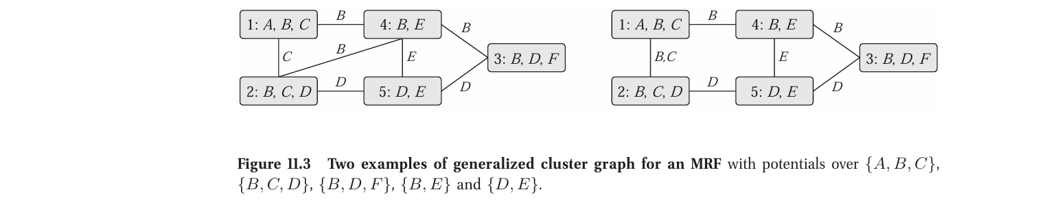
- Example: In 11.3a, $ C_1 $ and $ C_2 $ have $ B $ in common, but $ S_{1, 2} = \{ C \} $
Calibrated
A cluster graph is calibrated if for each edge $ (i - j) $, connecting the cluster $ C_i $ and $ C_j $:
$$
\boxed{ \sum_{C_i - S_{i, j}} \beta_i = \sum_{C_j - S_{i, j}} \beta_j }
$$
⚠️
That is, the two clusters agree on the marginal of variables in $ S_{i, j} $.
- clusters do not necessarily agree on the joint marginal of all variables they have in common,
- but only on those variables in the sepset $ S_{i, j} $
- as shown in the above example, some vars maybe in common but do not show up in sepset.
- Thus, this definition is weaker than cluster tree calibration.
ℹ️
However, if a calibrated cluster graph satisfies the RIP, then the marginal of a variable $ X $ is identical in all the clusters that contain it.
- marginal of $ X = \sum_{C_i - \{ X \}} \beta_i (C_i) $.
This means:
$ C_1 — C_2 — C_3 $
- $ C_1 = \{ X, Y \} $
- $ C_2 = \{ Y, Z \} $
- $ C_3 = \{ X, Z \} $
So $ X \notin C_2 $, during BP, clusters send messages over their shared variables (sepsets), however, there’s no way for information abt $ X $ to be passed bw $ C_1 $ and $ C_3 $
$ \Rightarrow C_1 $ and $ C_3 $ might converge to different marginals for $ X $.
When RIP is satisfied (+ calibrated)
- $ C_1 = \{ X, Y \} $
- $ C_2 = \{ X, Y, Z \} $
- $ C_3 = \{ X, Z \} $
Now all clusters that contain $ X $ have the same marignal distribution for $ X $.
$$
\sum_{C_i - \{ X \}} \beta_i = \sum_{C_j - \{ X \}} \beta_j
$$
❗
Calibration + RIP $ \Rightarrow $ Global consistency of marginals.
Cluster-Graph Belief Propagation

1. Initialize Cluster Graph
- Assign each factor $ \phi $ to a cluster.
- Construct initial potential
$$
\psi_i (C_i) = \prod_{\phi : \alpha (\phi) = i} \phi
$$
- Initialize all messages to be 1.
2. While graph is not calibrated, repeat
- select edge $ (i - j) $ and pass message
$$
\delta_{i \to j} (S_{i, j}) = \sum_{C_i - S_{i, j}} \psi_i \cdot \prod_{k \in Nb_i - \{ j \}} \delta_{k \to i}
$$
3. Compute
$$
\beta_i (C_i) = \psi_i \cdot \prod_{k \in Nb_i} \delta_{k \to i}
$$
- Repeat until when? When is the graph calibrated?
- How do I select the edge $ (i - j) $?
Properties of Cluster-Graph BP
Reparameterization
Similar to bp in clique tree, the convergence point represents a reparameterization of the original distribution.
- $ U $: generalized cluster graph over a set of factors $ \Phi $.
- $ \{ \beta_i \} $, $ \{ \mu_{i, j} \} $: set of beliefs and sepsets.
Theorem 11.4
𐰃𐰠𐰆𐰢
$ \tilde{P}_\Phi (\mathcal{X}) $
$$
\boxed{ = \frac{\prod_{i \in V_U} \beta_i[C_i]}{\prod_{(i - j) \in E_U} \mu_{i, j}[S_{i, j}]} }
$$
where $ \tilde{P}_\Phi (\mathcal{X}) = \prod \phi $ is the unnormalized distribution defined by $ \Phi $.
Proof
Recal:
$$
\beta_i = \psi_i \prod_{j \in Nb_i} \delta_{j \to i}.
$$
$$
\mu_{i, j} = \delta_{j \to i} \delta_{i \to j}.
$$
We now have
$$
\begin{align*}
\frac{\prod_{i \in V_U} \beta_i[C_i]}{\prod_{(i - j) \in E_U} \mu_{i, j}[S_{i, j}]} &= \frac{ \prod_{i \in V_U} \psi_i[C_i] \prod_{j \in Nb_i} \delta_{j \to i} [S_{i, j}] }{ \prod_{(i - j) \in E_U} \delta_{j \to i} [S_{i, j}] \delta_{i \to j} [S_{i, j}] }\\
&= \prod_{i \in V_U} \psi_i [C_i]\\
&= \prod_{\phi \in \Phi} \phi = \tilde{P}_\Phi (\mathcal{X})
\end{align*}
$$
This property shows that Cluster-Graph BP preserves all of the information about the original distribution.
Tree Consistency
Beliefs in general cluster graphs may not be exact marginals
From Theorem 10.4, if a set of calibrated beliefs match the marginals on a tree structure, then it also represents the joint distribution correctly.
$$
\beta_i (C_i) = P_\Phi (C_i)
$$
However,
- in loopy or general cluster graph, BP yields approximations, not guaranteed exact marginals of $ P_\Phi $.
- so can we say anything meaningful about these beliefs?
The idea is to select subtree $ T $ of general cluster graph $ U $ to investigate belief properties.
Subtree Marginals are consistent with subtree distributions

The selected subtree $ T $ is a subset of clusters and edges that
- together form a tree
- satisfies the RIP.
Example: In the figure, if we remove one of the clusters and its incident ediges, we are left with a proper cluster tree.
Note: RIP is not ncessarily as easy to achieve in general since removing some edges from the cluster graph may result in a graph that violates RIP relative to a variable $ \rightarrow $ need to remove additional edges, and so on.
Once selected a tree $ T $, we can think of it as defining a distribution
$$
P_T (\mathcal{X}) = \frac{\prod_{i \in V_T} \beta_i (C_i)}{\prod_{(i-j) \in E_T} \mu_{i, j} [S_{i, j}]}
$$
Tree consistency
If the cluster graph is calibrated $ \rightarrow $ so is $ T $ + satisfies RIP, we can apply Theorem 10.4
$$
\beta_i (C_i) = P_T (C_i)
$$
In English: the beliefs over $ C_i $ in the tree are the marginal of $ P_T $.
Analyzing Convergence
whether and when it converges?
Consider Standard sum-product message update rule
$$
\delta^\prime_{i \to j} \propto \sum_{C_i - S_{i, j}} \psi_i \cdot \prod_{k \in (Nb_i - \{ j \})} \delta_{k \to i}
$$
BP Operator
- takes all of the message $ \delta^t $,
- produces a new set of messages $ \delta^{t + 1} $ for the next step.
- $ t $: a particular iteration
- $ \Delta $: the space of all possible messages in the cluster graph.
𐰋𐰍𐰃𐰤
BP update operator $ G_{BP}: \Delta \mapsto \Delta $
$$
\boxed{ G_{BP} (\{ \delta_{i \to j} \}) = \{ \delta^\prime_{i \to j} \} }
$$
Contraction
A condition that guarantees convergence
- $ \alpha \in [0, 1) $: a number
- $ (\Delta, D) $: a metric space
- $ \Delta $: set of points we’re working with (in this case it is the space of all possible messages in the cluster graph).
- $ D(\delta, \delta^\prime) $: distance function.
An Operator $ G $ over a metric space $ (\Delta, D) $ is an $ \alpha $-contraction relative to the distance function $ D $ if,
for any $ \delta, \delta^\prime \in \Delta $,
$$
\boxed{ D(G(\delta); G(\delta^\prime)) \leq \alpha D(\delta, \delta^\prime) }
$$
An op is a contraction if its application to two points in the space is guaranteed to decrease the distance bw them by at least some constant $ \alpha < 1 $.
ℹ️
A contraction guarantees convergence to a fixed point, regardless of where you start from.
Fixed-point
Let $ G $ be an $ \alpha $-contraction of $ (\Delta, D) $. Then there is a unique fixed-point $ \delta^* $ st
$$
\boxed{ \lim_{n \to \infty} G^n (\delta) = \delta^* }
$$
TODO: Prove this
The contraction rate $ \alpha $ can be used to provide bounds on the rate of convergence of the algorithm to its unique fixed point: To reach a point that is guaranteed to be within $ \epsilon $ of $ \delta^* $, it suffices to apply $ G $ the following number of times:
$$
\log_\alpha \frac{\epsilon}{diameter(\Delta)}
$$
- $ diameter(\Delta) = \max_{\delta, \delta^\prime \in \Delta} D(\delta; \delta^\prime) $
Constructing Cluster Graphs
- Exact Inference: different clique trees $ \rightarrow $ different computational cost, same answer.
- Cluster Graph Approximation: different graphs $ \rightarrow $ different answers.
When selecting a cluster graph, we have to consider trade-offs bw cost and accuracy.
Pairwise Markov Networks

- A univariate potential $ \phi_i[X_i] $ over each var $ X_i $.
- A pairwise potential $ \phi_{(i, j)}[X_i, X_j] $ over some pairs of vars $ \rightarrow $ edges in Markov Net.
ℹ️
If we are willing to transform our variables, any distribution can be reformulated as a pairwise Markov network.
TODO: Exercise 11.10
Transformation from Markov Network to Cluster Graph
- For each potential, introduce corresponding cluster,
- put edges bw the clusters that have overlapping scope
- there’s an edge bw
- $ C_{(i, j)} $ that correspond to edge $ X_i - X_j $.
- and $ C_i, C_j $ that correspond to the univeriate factors over $ X_i $ and $ X_j $.
- Example: $ \boxed{ A_{1, 1} } — \boxed{ A_{1,1}, A_{1, 2} } — \boxed{ A_{1, 2} } $
Bethe Cluster Graph

- bipartite graph.
- first layer: “large” clusters
- one for each $ \phi \in \Phi $, scope is $ Scope[\phi] $.
- ensure family preservation property.
- second layer: “small” univeriate clusters
- one for each random variable.
- place an edge bw
- univariate cluster $ X $ on the second layer and
- each cluster in the first layer that includes $ X $.
Limitation the Bethe cluster graph: information between different clusters in the top level is passed through univariate marginal distributions $ \rightarrow $ interactions between variables are lost during propagations.
Other Entropy Approximations
Convex Approximations
Region Graph Approximations
Propagation with Approximate Messages
The Mean Field Approximation