General framework

• $ P (\mathcal{X}) $
• $ Y \subseteq \mathcal{X} $
• $ y \in Val(Y) $
• $ D = \{ \xi[1], \dots \xi[M] \}: M $ samples from $ P, \xi [i] \sim P $

Goal: Estimate $ P(Y) = y $.

Generally: Estimate the expectation of some $ f(x) $ relative to $ P $.

• To compute $ P(Y = y) $, choose $ f(\xi) = I \{ \xi (Y) = y \} $, $$ \begin{align*} E_{\xi \sim P}[f(\xi)] &\approx E_{\xi \sim D} [f(\xi)] \quad \text{(empirical approximation)}\\ &= \frac{1}{M} \sum_{1}^{M} f(\xi) = \frac{1}{M} \sum_{1}^{M} I\{ \xi(Y) = y \} \\ &= P(Y = y) \end{align*} $$

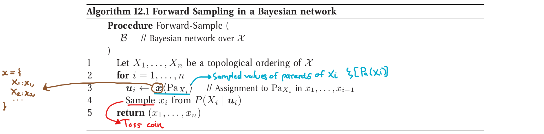
Forward Sampling

• Generate random samples $ \xi[1], \dots, \xi[M] $ from the distribution $ P(\mathcal{X}) $
• difficulties in generating samples from the posterior $ P(\mathcal{X} \mid e) $

FW-Sampling from a BN

Student Example

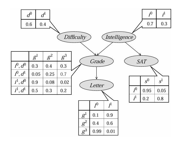
Sampling $ D $

toss a coin that land heads $ (d^1) $ 40% of the time and tails $ (d^0) $ 60%, assume tail landed $ \rightarrow \xi[D] = d^0 $

Sampling $ I $

assume $ \xi[I] = i^1 $

Sampling $ G $

Given $ d^0, i^1 \rightarrow $ Choose $ P(G \mid d^0, i^1) $ to sample.

…

Sampling from a Discrete Distribution

TODO: CS 109 or theprobabilitycourse sampling

Analysis of Error

• $ D = \{ \xi[1], \dots, \xi[M] \} $ generated via Forward-sampling
• Estimate $ P(Y = y) $
• $ I\{ \xi [m] (Y) = y \} \sim Bernoulli(P(y)) $, IID
  • because $ I = 1 $ with probability $ P (I = 1) = P (\xi [m] (Y) = y) = P(y) $ and $ 0 $ otherwise.

$ \rightarrow $ can estimate the expectation of any $ f $

$$ \hat{E_D} (f) = \frac{1}{M} \sum_{m = 1}^{M} f (\xi[m]) $$

FW-Sampling Estimator

In case of computing $ P(y) $, $ f $ counts # of times we see $ y $:

$$ \boxed{ \hat{P_D} (y) = \frac{1}{M} \sum_{m = 1}^{M} I \{ y[m] = y \} } \tag{12.2} $$

• $ y[m] $: denotes $ \xi [m] (Y) $ - the assignment to $ Y $ in the particle $ \xi [m] $

$ \Rightarrow $ apply the Hoeffding bound and Chernoff bound to show that this estimate is close to the truth with high probability.

Hoeffding bound

Measures the absolute error $ |\hat{P_D} - P(y)| $ $$ \boxed{ P_D (\hat{P_D} \notin [P(y) - \epsilon, P(y) + \epsilon]) \leq 2 e^{-2M \epsilon^2} } $$

• $ P_D (.) $: Probability of error (getting a bad sample set)
  • $ (\hat{P_D} \notin [P(y) - \epsilon, P(y) + \epsilon]) $: the estimator is $ \epsilon $ away from $ p $

We want: $$ P_D (\hat{P_D} \notin [P(y) - \epsilon, P(y) + \epsilon]) \leq \delta $$

• $ \delta $: failure tolarence, a small value.

Thus, we set: $$ \begin{align*} &\phantom{\leftrightarrow} 2 e^{-2M \epsilon^2} \leq \delta \\ &\Leftrightarrow -2M \epsilon^2 \leq \ln (\delta / 2)\\ &\Leftrightarrow \boxed{ M \geq \frac{\ln (2/s)}{2 \epsilon^2} } \end{align*} $$

Chernoff bound

$$ \boxed{ P_D (\hat{P_D} \notin P(y)(1 \pm \epsilon)) \leq 2 e^{-2M P(y) \epsilon^2/3} } $$

$$ \Leftrightarrow \boxed{ M \geq 3 \frac{\ln (2/ \delta)}{p \epsilon^3} } $$

Conditional Probability Queries

Conditional probabilities of the form $ P(y \mid E = e) $

Likelihood Weighting and Importance Sampling

Try: When sampling a node $ X_i $ whose value has been observed, set $ X_i $ to its observed value.

Assume evidence is $ s^1 $

• Sample $ D, I $ using naive fw-sampling process
• set $ S = s^1 $
• then sample $ G, L $.

$ \Rightarrow $ all of the samples will have $ S = s^1 $

Problem:

• The posterior probability of $ i^1 $ (smart student) should be higher when observed $ s^1 $ (high SAT score).
• But in fact, expected # of sample that have $ I = i^1 $ will still be 30%.

Ituition Example

$ E = \{ l^0, s^1 \} $

Assume

• sample $ D = d^1, I = i^0 $
• set $ S = s^1 $
• sample $ G = g^2 $
• set $ L = l^0 $

The probability that, given $ I = i^0 $, fw-sampling generated $ S = s^1 $: $$ P(s^1 \mid i^0) = 0.05 $$

The probability that, given $ G = g^2 $, fw-sampling generated $ L = l^0 $: $$ P(l^0 \mid i^0, g^2) = P(l^0 \mid g^2) \quad (\text{because } L \perp I \mid G) = 0.4 $$

Each of these events is the result of an independent coin toss. Thus the weight required for this sample to compensate for the setting of the evidence: $$ P(s^1, l^0 \mid i^0, g^2) = P(s^1 \mid i^0, g^2) \cdot P(l^0 \mid i^0, g^2) = P(s^1 \mid i^0) \cdot P(l^0 \mid g^2) = 0.05 \times 0.4 = 0.02 $$

Likelihood Weighting

The weight of samples are derived from the likelihood of the evidence accumulated throughout the sampling process.

This process generates a weighted particle.

Estimate a conditional probability $ P(y \mid e) $ using LW-Sample $ M $ times $ \rightarrow $ generate a set $ D = \{ \langle \xi[1], w[1] \rangle, \dots, \langle \xi[M], w[M] \rangle \} $ of weighted particles.

LW Estimator

$$ \boxed{ \hat{P_D} (y \mid e) = \frac{\sum_{m = 1}^{M} w[m] I\{ y[m] = y \}}{\sum_{m = 1}^{M} w[m]} } $$

This is a generalization of the one used for unweighted particles in (12.2).

Importance Sampling

Estimate the expectation of a function $ E[f(x)] $ relative to some target distribtuion $ P(X) $

• by generating samples $ x[1], \dots, x[M] $ from $ P $, then estimate

$$ \boxed{ E_P[f] \approx \frac{1}{M} \sum_{m = 1}^{M} f( x[m] ) } $$

Unormalized Importance Sampling

The sampling distribution $ Q $ is incorrect $ \rightarrow $ can’t avg the $ f $-value of the samples generated.

Observe $$ E_{P(X)} [f(X)] = E_{Q(X)} \left[f(X) \frac{P(X)}{Q(X)} \right] $$