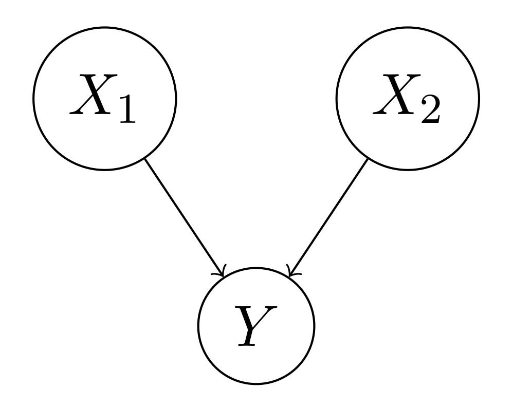
$X_1, X_2$: Causes,
$Y$: Effect.
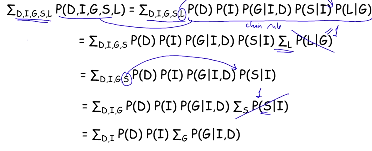
Because If we have the joint distribution, we can calculate any probability using the condition and marginal distribution
Consider a simple setting:
From $2^n - 1$ to $n$ is a dramatic reduction in the number of parameters, and the key point is:
The same applies to Conditional Indepence.
Consider a smaller picture: the joint distribution $ P(X_1, X_2, X_3, X_4) $. Using the chain rule,
$$ P(X_1, X_2, X_3, X_4) = P(X_4 \mid X_3, X_2, X_1) P(X_3 \mid X_2, X_1) P(X_2 \mid X_1) P(X_1) $$
If $ (X_4 \perp\!\!\!\perp X_1, X_2 \mid X_3) \in \mathcal{I}(P) $,then $ P(X_4 \mid X_3, X_2, X_1) = P(X_4 \mid X_3) $ $ \rightarrow $ # of required parameters for this CPD reduces from $ 2^3 = 8 $ to $ 2^1 = 2 $.
The joint distribution becomes
$$ P(X_1, X_2, X_3, X_4) = P(X_4 \mid X_3) P(X_3 \mid X_2, X_1) P(X_2 \mid X_1) P(X_1) $$
The total number of parameters reduces from $ 2^4 - 1 = 15 $ to $2 + 2^2 + 2 + 1 = 9$.
So it’s all about finding conditional independencies and factorize the joint distribution accordingly, but
$$ P(X_1, \dots, X_n) = \prod_i P(X_i \mid \text{Pa}_G(X_i)) $$

Example
 (a) A simple Bayesian network showing two potential diseases, Pneumonia and Tuberculosis,
All of the r.v are Boolean.
(b) The same Bayesian network, together with the conditional probability tables.

$X_1, X_2$: Causes,
$Y$: Effect.
From various causes predict the “downstream” efects , is predictive or causal reasoning.
Given $X_1$ and/or $X_2$, computing $P(Y \mid X_1), P(Y \mid X_2)$ and $P(Y \mid X_1, X_2)$.
We can condition on some variables (causes) and ask how that would change our probability $P(l^1)$.
$P(l^1 \mid i^0) \approx 0.39$, if we know that the student is not so smart, the probability of him getting reference letter goes down.
$P(l^1 \mid i^0, d^0) \approx 0.51$, if we now know that the class is easy, then the probability of the student getting high grade increases, thus he is more likely to get that refer letter.
From effect to cause , is called diagnostic or evidential reasoning.
Given $Y$, computing $P(X_1 \mid Y), P(X_2 \mid Y)$ and $P(X_1, X_2 \mid Y)$.
Student Example
We can condition on the Grade and ask what happens to the probability of its parents or its ancestors.
But now, with the additional evidence that the student has terrible grade $g^3$,
Explaining away is an instance of a general reasoning pattern called intercausal reasoning, that is reasoning between the causes with a common effect.
Student Example
Say, if a student gets low grade, he might not be so smart
On the other hand, if we now discover that the class is hard,
$\rightarrow$ we have explained away the poor grade via the dificulty of the class.
Example 2:
We have fever and a sore throat, and are concerned about mononucleosis.
Doctor then tells us that we have flu.
Having the flu does not prohibit us from having mononucleosis. Yet, having the flu provides an alternative explanation of our symptoms, thereby reducing substantially the probability of mononucleosis.