Deterministic CPDs
X is a deterministic function of its parents if there is a deterministic function $ f: Val(\text{Pa}_X) \mapsto Val(X) $ st
$$
\boxed{ P(x \mid \text{pa}_X) =
\begin{cases}
1 & x = f(\text{pa}_X) \\
0 & \text{otherwise}.
\end{cases} }
$$
binary OR Example
- $ Y, Z \in \{ 0, 1 \} $
- $ X = Y \lor Z $
| Y |
Z |
$ f(Y, Z) = Y \lor Z $ |
$ P(X = 1 \mid Y, Z) $ |
$ P(X = 0 \mid Y, Z) $ |
| 0 |
0 |
0 |
0 |
1 |
| 0 |
1 |
1 |
1 |
0 |
| 1 |
0 |
1 |
1 |
0 |
| 1 |
1 |
1 |
1 |
0 |
Continuous Variables
Some variables (e.g., position, velocity, temperature, pressure) are best modeled in a continuous space.
Discretization and its limitations
Example: A robot moving in 2D environment, where it position is described by x and y coordinates.
- Approximate position using a discrete grid with 15 cm per cell.
- Computational Infeasibility: Suppose each coordinate (x, y) has 1000 possible values $\rightarrow$ 1000 $\times$ 1000 = 1,000,000 possible discrete positions.
- Loss of Structure: Break the natural continuity of the robot’s position.
- Lack of Smooth Transitions:
- Basic continuity assumptions imply relationships between probabilities of nearby positions (i.e., smooth transitions),
- discrete models struggle to capture this property $\rightarrow$ Can not guarantee that nearby positions have similar probabilities.
BN requires the CPD $P(X \mid \text{Pa}_X)$ represent a distribution over $X$, for every assignment of values $\text{pa}_X$ to $\text{Pa}_X$.
- $X$ might be continous.
- Some of $X$’s parents might be continuous as well.
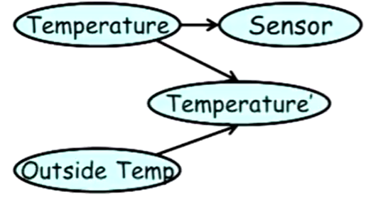
Example
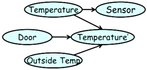
- Continuous Temperature (T) variable.
- Sensor (S) that measures the temperature in a room.
- This sensor is not perfect $\rightarrow$ the senor is around the right temperature but not quite.
Sensor S is normal distribution around T (true Temperature) with some standard deviation $\sigma$

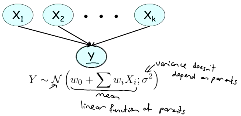
Linear Gaussian CPD

Let $Y$ be a continuous variable with continuous parents $X_1, \dots X_k$. $Y$ has a linear Gaussian model if there are parameters $w_0, \dots w_k$ and $\sigma^2$ such that:
$$
p(Y \mid X_1, \dots , X_k) = \mathcal{N}(w_0 + w_1X_1 + \dots + w_kX_k; \sigma^2).
$$
$$
\Leftrightarrow (Y \mid X_1, \dots, X_k) \sim \mathcal{N}(w_0 + \sum w_iX_i; \sigma^2).
$$
In vector notation,
$$
p(Y \mid \bf{x}) = \mathcal{N}(w_0 + \bf{w}^\intercal \bf{X}; \sigma^2).
$$
Y is a linear function of the variables $X_1, \dots X_k$, with the addition of Gaussian noise:
$$
Y = w_0 + w_1X_1 + \dots + w_kX_k + \epsilon,
$$
with $\epsilon \sim \mathcal{N}(0, \sigma^2). $
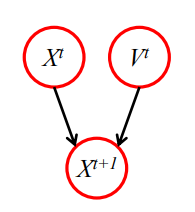
Example 1: Car Motion

Car moving along straight line
- At $t$ second
- Position: $X^t$ (at meter #510).
- Velocity: $V^t$ (15 m/s).
- Then at $t + 1$
- Position: $X^{t + 1} = X^t + V^t$ (expect: #525).
If there is stochasticity in motion, then it is much more realistic to describe the car’s position $X^{t + 1}$ using a Gaussian distribution:
$$
X^{(t + 1)} \sim \mathcal{N}(525, 5).
$$
Example 2: Temperature

$T$: The temperature now.
$T’$: The temperature soon. Depends on $T$ and $O$.
$P(T’)$ is a Gaussian around a mean that’s defined as a combination of T and O. One possible combination:
$$
T’ \sim \mathcal{N}(\alpha T + (1 - \alpha)O; \sigma{T}^2).
$$
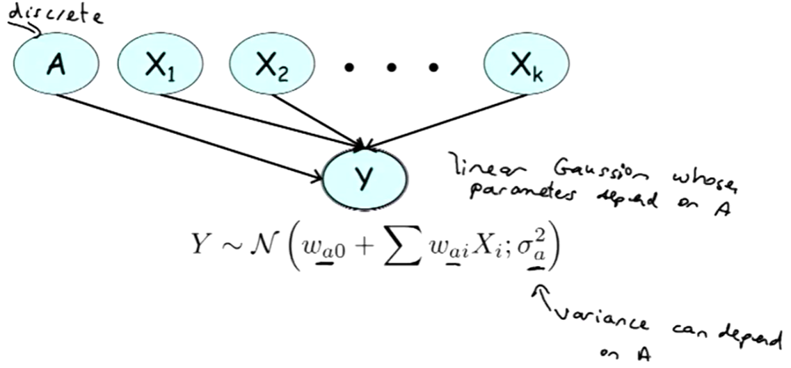
Conditional Linear Gaussian CPD

Let $Y$ be a continuous variable,
- its discrete parents $A = \{A_1, \dots A_m\}$.
- its continuous parents $X = \{X_1, \dots X_k\}$.
$Y$ has a conditional linear Gaussian (CLG) model if for every $a \in \text{Val}(A)$, there are
- $k + 1$ parameters $w_{a0}, \dots w_{ak}$
- and a variance $\sigma_a^2$ such that:
$$
p(Y \mid A = a, X) = \mathcal{N}(w_{a0} + \sum_{i=1}^{k}w_{ai}X_i; \sigma_a^2).
$$
Example: Temperature

$D$: The Door can be opened or closed.
- $T’ \sim \mathcal{N}(\alpha_0 T + (1 - \alpha_0)O; \sigma{0T}^2)$ if $D = 0$.
- $T’ \sim \mathcal{N}(\alpha_1 T + (1 - \alpha_1)O; \sigma{1T}^2)$ if $D = 1$.
⚠️
- Each combination of the discrete parents $A$ leads to a different set of coefficients $w_{a0}, \dots w_{ak} \rightarrow$ create a different Gaussian component (CPD of continuous var) with different mean and variance.
- $P(Y \mid X) = \sum_a P(A = a \mid X) \cdot \mathcal{N} (w_{a0} + \sum_{i=1}^k w_{ai}X_i; \sigma_a^2)$.
Conditional Linear Gaussian Network
𐰋𐰍𐰃𐰤
A Bayesian network is called a CLG network if every discrete variable has only discrete parents and every continuous variable has a CLG CPD.
❗
The CLG model does not allow for continuous variables to have discrete children.
Why?
- Discrete vars are represented using Conditional Probability Table (CPT), which requires a probability for each possible value of the discrete variable, given the values of its parents.
- If the parent is continuous, the number of possible values is infinite $\rightarrow$ need an infinite-sized CPT.
- This mean we would need to define $P(Y \mid X)$ as a continuous function of $X$ rather than a discrete table.

