Chapter 9: Exact Inference - Variable Elimination
PGMs represent joint probability distribution over a set of variables $\mathcal{X} \to$ use this representation to answer actual queries.
Queries
A query over a graphical model asks to compute simple statistics over the function such as its minimum or average value.
Conditional Probability Queries
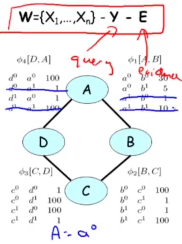
Given: Variables $\mathcal{X}$, Evidence $E = e$, Query $Y$.
Task: Compute $P(Y \mid E = e)$.
$$ \boxed{P(Y \mid E = e) = \frac{P(Y, e)}{P(e)}} $$
Let $W = \mathcal{X} - Y - E$ be variables that are neither query nor evidence (hidden variables).
$$ \boxed{P(Y, E = e) = \sum_{W} P(Y, E = e, W)} $$
$$ \boxed{P(e) = \sum_{Y, W} P(Y, E = e, W) = \sum_Y P(Y, E = e)} $$
Reduce factors
The sum can grow exponentially in the number of hidden variable.
Example
- $\mathcal{X} = \{X_1, \dots, X_5\}$, $X_i$ is binary variable.
- Evidence $E = {X_1 = 1}$.
- Query $Y = X_2$.
- $W = \mathcal{X} - Y - E = \{X_3, X_4, X_5\}$.
$$ P(Y = y, E = e) = \sum_{x_3, x_4, x_5} P(Y = y, X_1 = 1, \underbrace{X_3 = x_3, X_4 = x_4, X_5 = x_5}_{W}) $$
$\rightarrow$ Compute the joint probability for all 8 possible assignments of $x_3, x_4, x_5$.
In case of 20 variables? $2^{20}$.
Examples
Conditional probability inferences are often called Sum-Product: Sum over a product of factors.Student Example
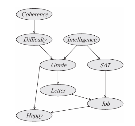
$$ P(J) = \sum_{C,D,I,G,S,L,H} \phi_C(C) \phi_D(C,D) \phi_I(I) \phi_G(G,I,D) \phi_S(S,I) \phi_L(L,G) \phi_J(J,L,S) \phi_H(H,G,J) $$
Observe evidences $I = i$ and $H = h$, plug in the original factors. $$ P(J \mid I = i, H = h) = \sum_{C,D,G,S,L} \phi_C(C) \phi_D(C,D) \phi_I(i) \phi_G(G,i,D) \phi_S(S,i) \phi_L(L,G) \phi_J(J,L,S) \phi_H(h,G,J) $$
$$ \tilde{P}(D) = \sum_{ABC} \phi_1(A, B) \times \phi_2(B, C) \times \phi_3(C, D) \times \phi_4(A, D) $$
Observe $A = a^0$, reduce factors by removing rows that are inconsistent with the observed evidence. $$ \tilde{P}(D, A = a^0) = \sum_{ABC} \phi^{\prime}_1(A = a^0, B) \times \phi_2(B, C) \times \phi_3(C, D) \times \phi^{\prime}_4(A = a^0, D) $$
Maximum a Posteriori (MAP)
Given: Variables $\mathcal{X}$, Evidence $E = e$, Query $Y = \mathcal{X} - E$.
Task: Compute $\text{MAP}(Y \mid E = e) = \text{argmax}_yP(Y = y \mid E = e)$.
- There might be more than one possible solution.
Max-Product
$$ P(Y \mid E = e) = \frac{P(Y, e)}{\underbrace{P(e)}_{\text{constant w.r.t Y}}} \propto P(Y, E = e) $$
$$ \begin{align*} P(Y, E = e) &= \frac{1}{\underbrace{Z}_{\text{const}}} \prod_k \phi^{\prime}_k(D^{\prime}_k) \\ &\propto \prod_k \phi^{\prime}_k(D^{\prime}_k) \end{align*} $$
$$ \boxed{\text{argmax}_Y P(Y \mid E = e) = \text{argmax}_Y \prod_k \phi^{\prime}_k (D^{\prime}_k)} $$
Analysis of Complexity
// TODO
Variable Elimination
Can use dynamic programming techniques to perform inference even for certain large and complex networks in a reasonable time.
Dynamic programming
- apply when the solution to a problem requires that we solve many smaller subproblems that recur many times.
- precomputing the solution to the subproblems,
- storing them,
- and using them to compute the values to larger problems.
Fibonacci
$ F_0 = 1 \\ F_1 = 1 \\ F_n = F_{n - 1} + F_{n - 2}. $
Recursive implementation
1(define (fib n)
2    (if (< n 2)
3        n
4        (+ (fib (- n 1)) (fib (- n 2)))))
$\rightarrow \mathcal{O}(2^n)$
Tail-Recursive implementation
1(define (fib n)
2    (define (fib-iter a b count)
3        (if (= count 0)
4            a
5            (fib-iter b (+ a b) (- count 1))))
6    (fib-iter 0 1 n))
$\rightarrow \mathcal{O}(n)$
VE’s core operations
Factor Product
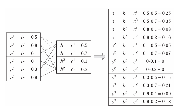
- $X, Y, Z$: r.v
- $\phi_1(X, Y)$, $\phi_2(Y, Z)$: factors
The product factor $\phi_1 \times \phi_2$ is a factor $\psi: \text{Val}(X, Y, Z) \to \mathbb{R}$ st:
$$ \boxed{\psi(X, Y, Z) = \phi_1(X, Y) \cdot \phi_2(Y, Z)} $$
Example: $\psi(A, B, C) = \phi_1(A, B) \cdot \phi_2(B, C)$.
Factor Marginalization
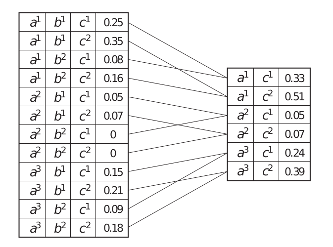
- $X$, $Y \notin X$: rv
- $\phi(X, Y)$: factor.
The factor marginalization of $Y$ in $\phi$, denoted $\sum_Y\phi$ is a factor $\psi$ over $X$ st:
$$ \boxed{\psi(X) = \sum_Y \phi(X, Y)} $$
summing out of $Y$ in $\psi$.
Properties of factor operations
Commutative $$ \boxed{\phi_1 \cdot \phi_2 = \phi_2 \cdot \phi_1 \quad \text{and} \quad \sum_X \sum_Y \phi = \sum_Y \sum_X \phi} $$
Associative $$ \boxed{(\phi_1 \cdot \phi_2) \cdot \phi_3 = \phi_1 \cdot (\phi_2 \cdot \phi_3)} $$
Exchange summation and product: If $X \notin \text{Scope}[\phi_1]$, then $$ \boxed{\sum_X(\phi_1 \cdot \phi_2) = \phi_1 \cdot\sum_X\phi_2} $$
VE General Idea
Eliminate-Var Z from $\Phi$
$\Phi = \{\phi_{X_i}\}^n_{i=1}$: Set of factors
- for each $\phi \in \Phi, \text{Scope}[\phi] \sub \mathcal{X}$.
$Z = \mathcal{X} - Y - E$.
- Write query in the sum-product form:
- If given Evidence $E = e$, we can reduce factors. $$ P(Y, e) = \phi^{*}(Y) = \sum_Z \prod_{\phi \in \Phi}\phi. $$
$\rightarrow$ this suggests an “elimination order” of latent variables to be marginalized.
- Iteratively
- Move all factors that does not involve $Z_k$ outside of $\sum_{Z_k}$ $$ \Phi^{\prime} = \{ \phi_i \in \Phi : \underbrace{Z_k \in \text{Scope}[\phi_i]}_{\text{all factors that involve Z}} \}. $$
$$ \psi = \prod_{\phi_i \in \Phi^{\prime}} \phi_i \quad ({\text{factor product}}). $$
- Perform sum out $Z$, getting a new term $\tau$
$$ \tau = \sum_{Z_k} \psi \quad ({\text{sum out $Z_k$ / marginalization}}). $$
- Insert the new term into the product
- Those $\prod_{\phi_i \in \Phi^{\prime}} \phi_i$ have been used, we don’t want to reuse them $\rightarrow$ take them out of the set of factors $\Phi$ and introduce the one created by sum-product.
$$ \Phi := (\Phi - \Phi^{\prime}) \cup { \tau }. $$
$$ P(Y, e) = \sum_{Z_1} \dots \sum_{Z_{k - 1}} \sum_{Z_{k + 1}} \dots \prod_{\phi \in \Phi}\phi \cdot \tau. $$
If $\phi$ are MN facors $\rightarrow$ normalize.
Example: Elimination in Chains
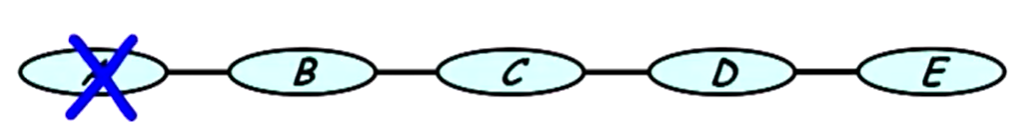
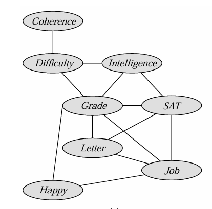
Example: Student BN
Compute $P(J)$. Elimination ordering: $C, D, I, H, G, S, L$.
- Eliminate: $C, D, I, H, G, S, L$.
$$ P(J) = \sum_{C,D,I,G,S,L,H} \phi_C(C) \phi_D(C,D) \phi_I(I) \phi_G(G,I,D) \phi_S(S,I) \phi_L(L,G) \phi_J(J,L,S) \phi_H(H,G,J) $$
$$ P(J) = \sum_{D,I,G,S,L,H} \phi_I(I) \phi_G(G,I,D) \phi_S(S,I) \phi_L(L,G) \phi_J(J,L,S) \phi_H(H,G,J) \underbrace{\sum_{C} \phi_C(C) \phi_D(C,D)}_{\tau_1 (D)} $$
- Eliminate: $D, I, H, G, S, L$.
$$ P(J) = \sum_{D,I,G,S,L,H} \phi_I(I) \phi_G(G,I,D) \phi_S(S,I) \phi_L(L,G) \phi_J(J,L,S) \phi_H(H,G,J) \tau_1 (D) $$
$$ P(J) = \sum_{I,G,S,L,H} \phi_I(I) \phi_S(S,I) \phi_L(L,G) \phi_J(J,L,S) \phi_H(H,G,J) \underbrace{\sum_{D} \phi_G(G,I,D) \tau_1 (D)}_{\tau_2 (G, I)} $$
- Eliminate: $I, H, G, S, L$.
$$ P(J) = \sum_{I,G,S,L,H} \phi_I(I) \phi_S(S,I) \phi_L(L,G) \phi_J(J,L,S) \phi_H(H,G,J) \tau_2 (G, I) $$
$$ P(J) = \sum_{G,S,L,H} \phi_L(L,G) \phi_J(J,L,S) \phi_H(H,G,J) \underbrace{\sum_{I} \phi_I(I) \phi_S(S,I) \tau_2 (G, I)}_{\tau_3 (G, S)} $$
$\dots$
- Eliminate: $L$.
$$ P(J) = \sum_{L}\tau_6 (J, L) $$
$$ P(J) = \tau_7 (J) $$
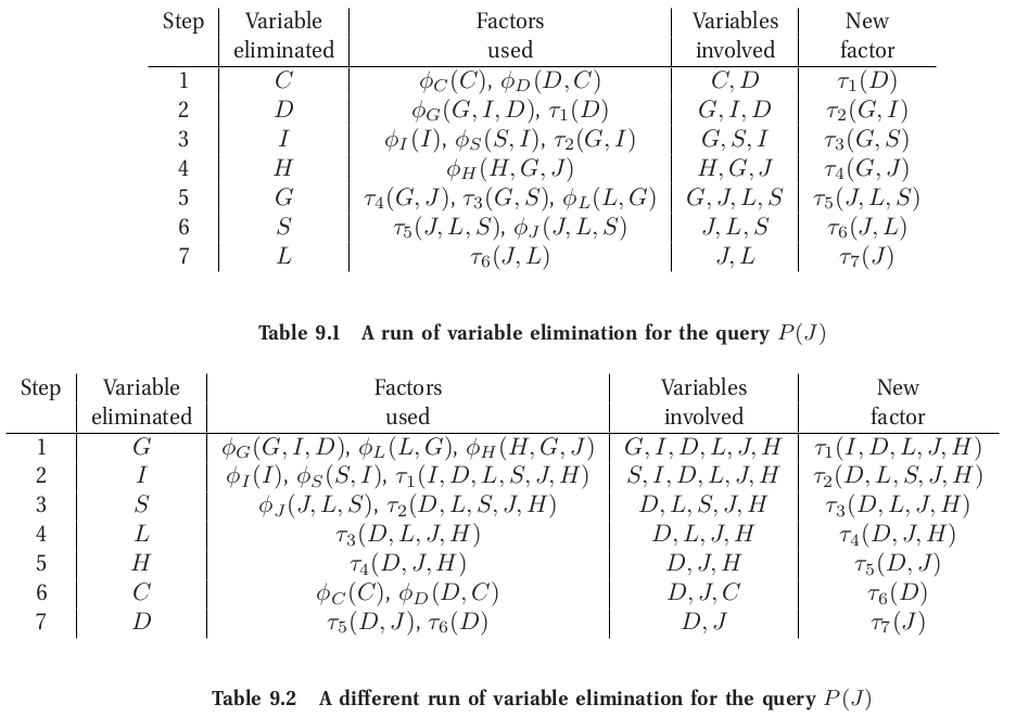
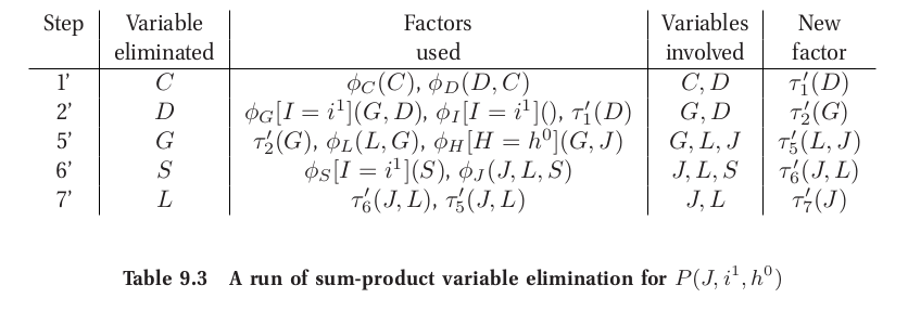
Compute $P(J , I = i^1, H = h^0 )$. Elimination ordering: $C, D, G, S, L$.
Reduced factors, eliminate as before.
$$ \sum_{L, S, G,, D, C} \phi_J(J, L, S) \phi_L(L, G) \phi_S^{\prime}(S) \phi_G^{\prime}(G, D) \phi_H^{\prime}(G, J) \underbrace{\phi_I()}_{\phi_I(i^1): \text{ constant}} \phi_D(C, D) \phi_C(C) $$
Semantics of Intermediate Factors
Factors are not always correspond to marginal or conditional probabilities in the network.
Complexity of VE
$$ \psi_k(X_k) = \prod_{i = 1}^{m_k}\phi_i \quad \text{(factor product)} $$
- $m_k$: factors that involve $Z$.
$$ \tau_k(X_k - \{Z\}) = \sum_{Z} \psi_k(X_k) \quad \text{(marginalization)} $$
Factor Product Complexity
- $ m_k $: number of involved factors.
$$ \psi_k(X_k) = \prod_{i = 1}^{m_k}\phi_i $$
-
Number of rows in the resulting table: $N_k = |\text{Val}(X_k)| \rightarrow$ $3 \times 2 \times 2 = 12$
-
Each row: $m_k - 1$ products $\rightarrow$ 2 in this case.
$$ \text{Cost: }\boxed{(m_k - 1)N_k}\text{ multiplications} $$
Factor Marginalization Complexity
$$ \tau_k(X_k - \{Z\}) = \sum_{Z} \psi_k(X_k) $$
- Each row used exactly once
$$\boxed{N_k = |\text{Val}(X_k)|} \text{ additions}$$
Complexity
- Assume
- $m$ factors and $n$ rv.
- $m = n$ for Bayesian networks (one factor/CPD for every var).
- can be larger for Markov networks.
- run the algorithm until all variables are eliminated.
- At each elimination step generate exactly one factor $\tau_k$.
- At most $n$ elimination steps.
- each step eliminates one variable.
- Total number of factors that entered $ \Phi $:
$$ m^* \leq m + n $$
- Product operations:
$$
\sum_k (m_k - 1) N_k \leq \sum_k (m_k - 1) N \leq (m + n)N = \mathcal{O}(mN)
$$
- $ N = \text{max}(N_k) = $size of the largest factor.
- sum of different elimination steps.
- each factor multiply at most once.
- Sum operations: $$ \sum_k N_k \leq nN $$
- Total work is linear in $N$ and $m$:
$$ \boxed{ \underbrace{\sum_k (m_k - 1)N_k}_{\text{products}} + \sum_k N_k \leq (m + n)N = \mathcal{O}((m + n)N) = \mathcal{O}(mN) } $$
- $N_k = |\text{Val}(X_k)| = \mathcal{O}(d^{r_k})$: Number of values in a factor.
- $d = max(|\text{Val}(X_i)|)$: each variable has no more than $d$ values.
- $r_k = |X_k|$: $\psi_k$ has a scope that contains $r_k$ variables.
Complexity and Graph Structure: VE
Elimination as Graph Transformation
Moralization
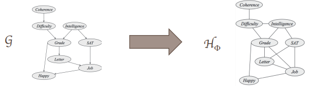
Moralization procedure
- Starting from an input DAG
- Connect nodes if they share a common child
- Make directed edges to undirected edges
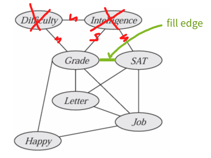
Fill Edge
Eliminating a variable $X$:
- Constructing a factor $\psi$ over $X$ and its neighbors $Y$.
- Then eliminate $X$ to new factor $\tau$ over $Y$.
To reflect this in graph:
- Add edges (called fill edges) between all pairs in $ Y $ if not already present.
- Eliminate $X$ + remove its incident edges.
Example
$$ \begin{align*} &\phi_C(C) \phi_D(C,D) \phi_I(I) \phi_G(G,I,D) \\ &\phi_S(S,I) \phi_L(L,G) \phi_J(J,L,S) \phi_H(H,G,J) \end{align*} $$
$$ \tau_1(D) = \sum_C \phi_C(C)\phi_D(C, D) $$
$$ \tau_2(G, I) = \sum_D \phi_G(G, I, D)\tau_1(D) $$
$$ \tau_3(S, G) = \sum_I \phi_S(S, I)\phi_I(I)\tau_2(G, I) $$
Induced Graph
The induced graph $ \mathcal{I}_{\Phi, \alpha} $ over factors $ \Phi $ and ordering $ \alpha $:
- Undirected graph.
- $ X_i $ and $ X_j $ are connected if they appeared in the same factor during a run of the VE algorithm using $ \alpha $ as the ordering.
Induced Graph and Clique Tree Theorem
Theorem 9.6
-
The scope of every factor produced during VE is a clique in the induced graph.
-
Every (maximal) clique in the induced graph is a factor produced during VE.
Proof (1)
Induced Width
- $ K $: undirected or directed graph.
- $ \mathcal{I}_{K, \alpha} $: Graph induced by applying VE to $ K $ using order $ \alpha $.
- $ w_{K, \alpha} $: Induced width (width of the induced graph).