Chapter 2: Probability - Univariate Models
What is probability?
Bayesian interpretation of probability: used to quantify our uncertainty or ignorance about something $\rightarrow$ related to INFORMATION rather than repeated trials.
Types of uncertainty
epistemic (model) uncertainty
- epistemology is the philosophical term used to describe the study of knowledge.
- due to our ignorance of the underlying hidden causes or mechanism generating our data.
aleatoric (data) uncertainty
- aleatoric means “dice”.
- arises from intrinsic variability, which cannot be reduced even if we collect more data.
Probability as an extension of logic
Probability of a conjunction of two events
Joint probability
Random Variables
Quantiles
Recall
A function $f$ has an inverse $f^{-1}$ if: $$ f(f^{-1}(y)) = y \text \quad { and } \quad f^{-1}(f(x)) = x $$
But this only work if $f$ is bijective:
- Injective (one-to-one): $f(x_1) = f(x_2) \Rightarrow x_1 = x_2$
- Surjective (onto): The range of $f$ covers the entire domain
Monotonically increasing $$ x_1 < x_2 \Rightarrow f(x_1) \leq f(x_2) $$ Strictly increasing $$ x_1 < x_2 \Rightarrow f(x_1) < f(x_2) $$
If cdf $F$ is strictly monotonically increasing, it has an inverse CDF or quantile function. $$ \boxed{F^{-1}(p) = \text{inf}\{x \in \mathbb{R}: F (x) \geq p\} \quad \text{for } p \in (0, 1)} $$
Or
$$ F^{-1}(p) = x \text{ such that } P_X(X \leq x) = p $$
Sets of related random variables
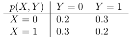
marginal distribution $$ \boxed{p(X = x) = \sum_y p(X = x, Y = y)} $$
conditional distribution (product rule) $$ \boxed{p(Y = y \mid X = x) = \frac{p(X = x, Y = y)}{p(X = x)}} $$
$$ \Rightarrow p(x, y) = p(x)p(y \mid x) $$
chain rule: Extend the product rule to $D$ variables $$ \boxed{p(x_{1: D}) = p(x_1)p(x_2 \mid x_1)p(x_3 \mid x_1, x_2)p(x_4 \mid x_1, x_2, x_3) \dots p(x_D \mid x_{1:D - 1})} $$
Independence and conditional independence
marginally independent $$ \boxed{X \perp Y \Leftrightarrow p(X, Y) = p(X)p(Y)} $$
$X_1, \dots, X_n$ are mutually independent if the joint can be written as a product of marginals for all subsets $\{X_1, \dots, X_m\} \sub \{X_1, \dots, X_n\}$ $$ \boxed{p(X_1, \dots, X_m) = \prod_{i = 1}^m p(X_i)} $$
mutually independent
$X_1, X_2, X_3$ are mutually indepedent if
- $p(X_1, X_2, X_3) = p(X_1)p(X_2)p(X_3)$.
- $p(X_1, X_2) = p(X_1)p(X_2)$.
- $p(X_2, X_3) = p(X_2)p(X_3)$.
- $p(X_1, X_3) = p(X_1)p(X_3)$.
Unconditional independence is rare, because most variables can influence most other variables via other variables.
conditionally independent (CI) $$ \boxed{X \perp Y \mid Z \Leftrightarrow p(X, Y \mid Z) = p(X \mid Z)p(Y \mid Z)} $$
Moments of a distribution
Various summary statistics that can be derived from a probability distribution.
First Moment: Mean
Discrete
$$ \boxed{E[X] = \sum_{x \in \mathcal{X}} x \, p(x) \, dx} $$
Continuous
$$ \boxed{E[X] = \int_{\mathcal{X}} x \, p(x) \, dx} $$
linearity $$ \boxed{\mathbb{E}[aX + b] = a\mathbb{E}[X] + b} $$
- For a set of $n$ r.v
$$
\boxed{\mathbb{E}\left[\sum_{i = 1}^n X_i\right] = \sum_{i = 1}^n \mathbb{E}[X_i]}
$$
If they are independent
$$
\boxed{\mathbb{E}\left[\prod_{i = 1}^n X_i\right] = \prod_{i = 1}^n \mathbb{E}[X_i]}
$$
explain
$\mathbb{E}[XY] = \int xy \, P_{XY}(x, y) \, dx \, dy$.
If $X \perp Y \Rightarrow P_{XY}(x, y) = P_X(x)P_Y(y)$
Second Moment: Variance
$$ \begin{align*} \mathbb{V}[X] &\triangleq \boxed{\mathbb{E}\left[(X - \mu)^2\right]} \\ &= \int (x - \mu)^2 p(x) \, dx \\ \quad &= \int x^2 p(x) \, dx + \mu^2 \int p(x) \, dx - 2\mu \int x p(x) \, dx = \boxed{\mathbb{E}\left[X^2\right] - \mu^2} \end{align*} $$ from which we derive the useful result $$ \boxed{\mathbb{E}[X^2] = \sigma^2 + \mu^2} $$
standard deviation $$ \boxed{\sigma = \sqrt{\mathbb{V}[X]}} $$
linearity
$$
\boxed{\mathbb{V}[aX + b] = a^2 \mathbb{V}[X]}
$$
verify
$\mathbb{V}[aX + b] = \mathbb{E}\left[(aX + b - \mathbb{E}[aX + b])^2\right] = \mathbb{E}\left[(aX - \mathbb{E}[aX])^2\right] = a^2 \mathbb{V}[X]$
- $n$ independent rv $\rightarrow$ the variance of their sum is given by the sum of their variances $$ \boxed{\text{Var}\left( \sum_{i=1}^{n} X_i \right) = \sum_{i=1}^{n} \text{Var}[X_i] } $$
$$ \begin{align*} \text{Var}\left( \prod_{i=1}^{n} X_i \right) &= E\left[ \left( \prod_{i=1}^{n} X_i \right)^2 \right] - \left( E\left[ \prod_{i=1}^{n} X_i \right] \right)^2 \\ &= E\left[ \prod_{i} X_i^2 \right] - \left( \prod_{i} E[X_i] \right)^2 \\ &= \prod_{i} E[X_i^2] - \prod_{i} E[X_i]^2 \\ &= \prod_{i} \left( \text{Var}[X_i] + (E[X_i])^2 \right) - \prod_{i} E[X_i]^2 \\ &= \boxed{\prod_{i} \sigma_i^2 + \mu_i^2 - \mu^2} \end{align*} $$
Mode of a distribution
the value with the highest probability mass / density: $$ \boxed{ x^* = \argmax_x p(x) } $$
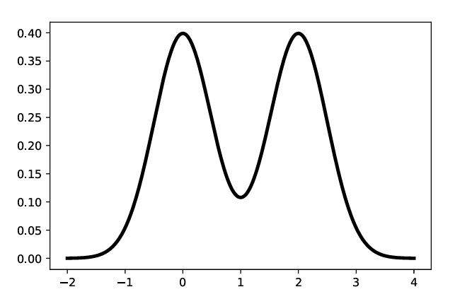
If the distribution is multimodal, this may not be unique.
Example: mixture of two 1d Gaussian, $$ p(x) = 0.5 \mathcal{N} (0, 0.5) + \mathcal{N} (2, 0.5) $$