Continuous Random Variables and PDFs
𐰋𐰍𐰃𐰤
A random variable (takes values from a continuous set) is continuous if it can be described by a PDF.
PDF
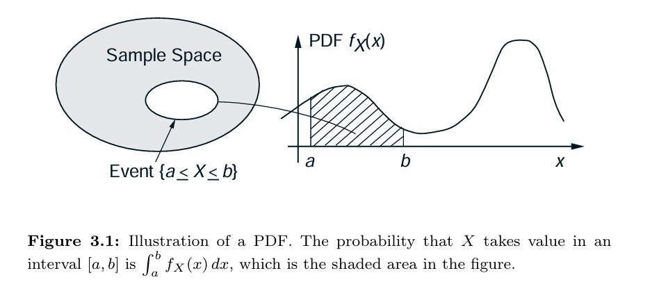
The area under the graph of the PDF.
$$
\boxed{P(a \leq X \leq b) = \int_a^b f_X \, (x) \, dx}
$$
To qualify as an PDF, $f_X(x) \geq 0$ for every $x$, and $f_X$ must satisfy the normalize equation:
$$
\int_{- \infty}^{\infty} f_X(x) \, dx = P(- \infty < X < \infty) = 1
$$
⚠️
For any single value $a$, $P(X = a) = \int_a^a \, f_X(x) \, dx = 0$.
Thus
$$
P(a \leq X \leq b) = \underbrace{P(X = a)}_0 + \underbrace{P(X = b)}_0 + P(a < X < b) = P(a < X < b).
$$
Jumps in the CDF correspond to points $x$ for which $P(X = x) > 0$. Thus the fact that the CDF does not have jumps is consistent with the fact that $P(X = x) = 0$ for all $x$.
Probability of small interval
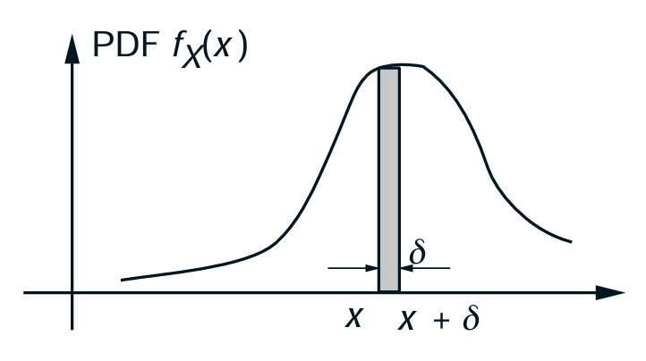
$\delta > 0$, small
$$
\boxed{\mathbf{P}(x < X < x + \delta) = \int_x^{x + \delta} f_X(t) \, dt \approx f_X(x) \cdot \delta}
$$
$$
\Rightarrow f_X(x) = \frac{P(x \leq X \leq x + \delta)}{\delta} = \frac{\text{Probability mass}}{\text{Unit length}}
$$
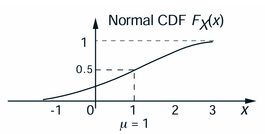
Cumulative Distribution Function
The CDF $F_X(x)$ “accumulates” probability “up to” the value of $x$.
$\{X \leq x\}$ is always an event $\Rightarrow$ Any random variable associated with a given probability model has a CDF, regardless of whether it is discrete, continuous, or other.
Properties of CDF
continuously varying form
-
$F_X$ is monotonically nondecreasing:
$$
\text{if } x \leq y \text{, then } F_X(x) \leq F_X(y).
$$
-
$F_X$ tends to 0 as $x \to -\infty$, and to 1 as $x \to \infty$.
-
the PDF and the CDF can be obtained from each other by integration or differentiation
$$
\boxed{F_X(x) = \int_{-\infty}^{x}f_X(t) \, dt}
$$
$$
\boxed{f_X(k) = \frac{dF_X}{dx} (x) = F^{\prime}_X(x)}
$$
❗
Once we know the CDF of a random variable, we can calculate anything we might want to calculate.
$P(a < X < b)$
For all $a \leq b$,
$$
\boxed{P(a < X \leq b) = P(X \leq b) - P(X \leq a) = F_X(b) - F_X(a)}
$$
Why is CDF prefered?
Gaussian (normal) PDF
Important in the theory of probability: Centrail limit theorem.
If you have a phenomenon in which you measure a certain quantity, but that quantity is made up of lots and lots of random contributions.
Then your random variable is actually the sum of lots and lots of independent little random variable. And no matter what kind of distribution the little random variables have, their sum will turn out to have approximately a normal distribution.
$\rightarrow$ This makes the normal distribution to arise very nartually in lots and lots of context. Whenever you have noise that’s comprise of lots of different independent pieces of noise, then the end result will be a random normal variable.
Standard normal (Gaussian) random variables
- So what is standard normal?
𐰋𐰍𐰃𐰤
STANDARD NORMAL
$$X \sim \mathcal{N}(0, 1): f_X(x) = \frac{1}{\sqrt{2\pi}} e^{-x^2/2}$$
why $\frac{1}{\sqrt{2\pi}}$ ?
$\int_{-\infty}^{\infty}e^{-x^2/2} , dx = \sqrt{2\pi}$

- $\mathbb{E}[X] = 0$
- $\text{Var}(X) = \mathbb{E}[X^2] - 0 = 1$
Integrate by parts
$
u = x
$
$
dv = xe^{-x^2/2} \, dx \rightarrow v = -e^{-x^2/2}
$
$$
\int udv = uv - \int vdu = \frac{1}{\sqrt{2\pi}}(-xe^{-x^2/2}\Big|_{-\infty}^{\infty} + \int_{-\infty}^{\infty} e^{-x^2/2} \, dx) = 0 + 1 = 1
$$
Example 3.10: Memorylessness of the exponential PDF